User Manual¶

Installation¶

There are two methods to install AdaptivePELE [APELE], from PyPI (recommended) or directly from source.

To install from PyPI simply run:

pip install AdaptivePELE

To install from Conda run:

conda install -c conda-forge -c nostrumbiodiscovery adaptive_pele

You can use a container image to run AdaptivePELE, using either Docker or Singularity (recommended). Note that when using PELE as propagator, you will need access to a PELE license, please contact Nostrum Biodiscovery (http://nostrumbiodiscovery.com) for that. To build a singularity image with PELE support, you an follow this steps:

git clone https://github.com/AdaptivePELE/AdaptivePELE.git
cd docker
cp /path/to/pele_image.sif pele.sif
singularity build adaptivepele.sif AdaptivePELE.def

There is a docker image available, but taht does only allow to run MD simulaitons using OpenMM. You can get it from the dockerhub:

docker pull cescgina/adaptivepele_md

Note that running simulations from this container would require some tweaking, as you need to mount a volume to give access to the input files, as well as the output location, which is why we recommend to use singularity. You can obtain a singularity image from the docker one running:

singularity pull adaptivepele_md.sif docker://cescgina/adaptivepele_md

To install from source, you need to install the depencies:

git clone https://github.com/AdaptivePELE/AdaptivePELE.git
cd AdaptivePELE
pip install --requirement requirements.txt

and compile cython files in the same folder with:

python setup.py install

Also, if AdaptivePELE was not installed in a typical library directory, a common option is to add it to your local PYTHONPATH:

export PYTHONPATH="/location/of/AdaptivePELE:$PYTHONPATH"

Overview¶

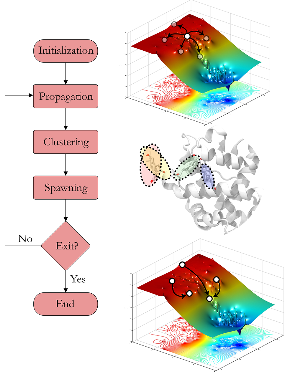
This page tries to give an overview of AdaptivePELE, enough to get it up and running. The program aims to enhance the exploration of standard molecular simulations by iteratively running short simulations, assessing the exploration with a clustering, and spawning new trajectories in interesting regions using the multi-armed bandit as a framework. The algorithm can be summarized in the flow diagram shown below:

Control file outline¶

AdaptivePELE is a Python program called with a parameter: the control file.

python -m AdaptivePELE.adaptiveSampling controlFile.conf

The control file is a JSON document that permits tuning its behavior. It contains 4 blocks: the general parameters, simulation parameters, clustering parameters and spawning parameters. The first block refers to general parameters such as the output path, initial structures, or whether to restart (resume) a simulation. The other three blocks configure the three iterative steps of an adaptive run, and have a {"type":str, "params":{}, "optionalClasses":{}} structure. Namely, the simulation block chooses and tunes the propagation algorithm, typically PELE, the clustering block tunes the clustering method, cluster sizes… and the spawning block selects the strategy to choose the most interesting structures.

{
    "generalParams" : {},
    "simulation": {"type":str, "params":{}},
    "clustering": {"type":str, "params":{}},
    "spawning": {"type":str, "params":{}}
}

GeneralParams block¶

These parameters control the general aspects of the simulation, such as the initial structures or the output path. For example, if you consider that a simulation did not explore the energy landscape sufficiently, it can be automatically resumed. In this case, if you change the clustering parameters from the previous run, it will need the trajectory files to recluster all snapshots. Otherwise, it is enough with the automatically handled clustering objects. If you want to test the effect of using a particular cluster threshold or spawning parameter (see below), using debug=true may be a great option.

Parameters¶

The general parameters block has five possible fields:

restart (boolean, default=True): This parameter specifies whether you want to continue a previous simulation or not. It requires the last epoch’s clustering object, which is stored as a binary file to optimize disk usage.
debug (boolean, default=False): Run adaptive in debug mode, without calling any propagation algorithm. Typically used to tinker with the clustering/spawning.
outputPath (string, mandatory): The path where the results of the simulation will be written
initialStructures (list, mandatory): The path(s) to the intial structure(s)
writeAllClusteringStructures (boolean, default=False): Whether to write all the cluster center structures as pdbs. Setting it to True is inneficient, and cluster center structures can still be recovered from the binary clustering object.

Additionaly, it can also have a nativeStructure parameter, a string containing the path to the native structure. This structure will only be used to correct the RMSD in case of symmetries. The symmetries will also have to be specified (see clustering block).

Example:

"generalParams" : {
    "restart": false,
    "debug" : false,
    "outputPath":"simulationOutput",
    "nativeStructure" : "nativeStructure.pdb",
    "initialStructures" : ["initial1.pdb", "initial2.pdb"]
}

Simulation block¶

Currently, there are three implemented simulation types:

pele. PELE is a great tool to efficiently explore the energy landscape. Parameters have been optimized for its use.
test. The test type has no real use outside of testing.
MD Run molecular dynamics using the OpenMM [OPENMM] library.

Templetized PELE control file¶

In order to run adaptivePELE, PELE control file needs to be templetized. In particular:

MultipleComplexes”: AdaptivePELE requieres the use of multiple complexes: "MultipleComplex": [ $COMPLEXES ]
seed: The seed needs to be templetized: "seed": $SEED
outputPath: The output path needs to be changed for: "reportPath": "$OUTPUT_PATH/report"
numberOfPeleSteps: The number of pele steps needs to be templetized as "numberOfPeleSteps": $PELE_STEPS

Optionally other fields might be templetized as well:

fixedCenter: The center of the simulation box is templetized as "fixedCenter": $BOX_CENTER
radius: The radius of the simulation box is templetized as "radius": $BOX_RADIUS
reportName: The name of the report file is templetized as "reportPath": "$OUTPUT_PATH/$REPORT_NAME". Note that the value of the reportName is not a parameter of the simulation block, but is given by the reportFilename option of the spawning block
trajectoryName: The name of the trajectory file is templetized as "trajectoryPath": "$OUTPUT_PATH/$TRAJECTORY_NAME"

PELE Parameters¶

When using PELE as a propagator, the following parameters are mandatory:

iterations (integer, mandatory): Number of adaptive sampling iterations to run
processors (integer, mandatory): Number of processors to use with PELE
peleSteps (integer, mandatory): Number of PELE steps in a epoch (iteration)
seed (integer, mandatory): Seed for the random number generator
controlFile (string, mandatory): Path to the templetized PELE control file (see below)

Optionally, you can also use the following parameters:

data (string, default=MareNostrum or Life cluster path): Path to the Data folder needed for PELE
documents (string, default=MareNostrum or Life cluster path): Path to the Documents folder needed for PELE
executable (string, default=MareNostrum or Life cluster path): Path to the Pele executable folder
trajectoryName (string, default=None): Name of the trajectories to substitute in the PELE control file
modeMovingBox (string, default=None, possible values={unbinding, binding}): Whether to dynamically set the center of the simulation box along an exit or entrance simulation
boxCenter (list, default=None): List with the coordinates of the simulation box center
boxRadius (int, default=20): Value of the simulation box radius (in angstroms)
runEquilibration (bool, default=False): Whether to run a short equilibration or burn-in simulation for each initial structure
equilibrationLength (int, default=50): Number of steps for the equilibration run
equilibrationMode (string, default=”equilibrationSelect”): Choose the mode of the equilbration run, equilibrationSelect selects one of the structures as a representative as a function of distance and energy, while equilibrationLastSnapshot selects the last snapshot of each trajectory as representatives and equilibrationCluster clusters the output of the 25% best energy structures in the equilibration by the center of mass.
numberEquilibrationStructures (int, default=10): Number of clusters to obtain from the equilibrationCluster structure selection (see equilibrationMode for more details)
equilibrationBoxRadius (float, default=2.0): Value of the simulation box radius for the equilibration (in angstroms)
equilibrationRotationRange (float, default=0.05): Value of the rotation magnitude in the equilibration simulation
equilibrationTranslationRange (float, default=0.5): Value of the translation magnitude in the equilibration simulation
useSrun (bool, default=False): Whether to use srun to launch the PELE simulation instead of mpirun. Using srun allows a finer control over the resources used and might be helpful to deal with different cluster configurations or SLURM installations.
srunParameters (string, default=None): String with parameters to pass to srun, if not specified it will just run without any parameters, it is important to avoid whitspaces both at the beginning and end of the string.
mpiParameters (string, default=None): String with parameters to pass to mpirun, if not specified it will just run without any parameters, it is important to avoid whitspaces both at the beginning and end of the string.
time (float, default=None): Time limit for the simulation (in seconds), if no value is specified simulation is run until the number of steps in peleSteps is finished

MD Parameters¶

When using MD as a progagator, the following parameters are mandatory:

iterations (integer, mandatory): Number of adaptive sampling iterations to run
processors (integer, mandatory): Number of processors to use
productionLength (integer, mandatory): Number of time steps in a epoch (iteration)
seed (integer, mandatory): Seed for the random number generator
reporterFrequency (integer, mandatory): Frequency to write the report and trajectories (in time steps, see timeStep property)
numReplicas (integer, mandatory): Number of replicas to run (see Running AdaptivePELE with GPUs section), each replica will run the same number of trajectories, calculated as t = p/n, where t is the number of the trajectories per replica, p is the number of processors and n is the number of replicas

Optionally, you can also use the following parameters:

equilibrationLengthNVT (int, default=200000): Number of steps for the constant volume equilibration run (default corresponds to 400 ps)
equilibrationLengthNPT (int, default=500000): Number of steps for the constant pressure equilibration run (default corresponds to 1 ns)
timeStep (float, default=2): Value of the time step for the integration (in femtoseconds)
boxCenter (list, default=None): List with the coordinates of the simulation box center. When using a simulation box in a run with multiple ligands, please ensure that the ligandsToRestrict parameter is correctly set.
boxRadius (float, default=20): Radius of the spherical box the ligand will be restrained to (in angstroms). Note that when using the spherical box restraint only xtc trajectories are supported.
ligandName (str or list, default=None): Ligand residue name in the PDB for all residues that must be parametrised, starting from version 1.6.3 more than one ligand can be specified
ligandCharge (integer or list, default=None): Charge of the ligand for all residues that must be parametrised, starting from version 1.6.3 more than one ligand can be specified
WaterBoxSize (float, default=8): Distance of the edge of the solvation box from the closest atom (in angstroms)
nonBondedCutoff (float, default=8): Radius for the nonBonded cutoff of the long-range interactions (in angstroms)
temperature (float, default=300): Temperature of the simulation (in Kelvin)
runningPlatform (str, default=CPU): Platform on which to run the simulation, options are {CPU, CUDA, OpenCL, Reference}, see openmm documentation for more details
minimizationIterations (float, default=2000): Number of time steps to run the energy minimization
devicesPerTrajectory (int, default=1): Number of gpus to use for each trajectory, this parameter only applies if using the CUDA platformn. Note that devicesPerTrajectory*numReplicas should correspond to the number of gpus per node that you have available
maxDevicesPerReplica (int, default=None): Number of maximum gpus available per replica, this parameter is necessary if one wants to oversubscribe the gpus, i.e. run more than one trajectory in the same device
constraintsMinimization (float, default=5.0): Value of the constraints for the minimization (in kcal/(mol*A²)), see Equilibration procedure in MD section for more details on the equilibration procedure
constraintsNVT (float, default=5.0): Value of the constraints for the NVT equilibration (in kcal/(mol*A²))
constraintsNPT (float, default=0.5): Value of the constraints for the NPT equilibration (in kcal/(mol*A²))
format (str, default=xtc): Format of the trajectory file, currently we support dcd and xtc, note however that due to issues with the xtc library in mdtraj writing xtc files might not be problematic unless you are currently using the latest mdtraj code (this means version > 1.9.2 at the moment this was written)
constraints (list, default=None): List of constraints between atoms to establish in a simulation. The constraints must be specified as a list in the following format (see Control File Examples section for an example on how to set constraints. Note: the distance of the constraints must be specified in angstroms):
```
["atom1:res1:resnum1", "atom2:res2:resnum2", distance]
```
Note 2: Histidines present in constraints should be named HIS regardless of their protonation state, see Input preparation for MD section for more details on histidines naming.
boxType (str, default=sphere): Type of box to use, it can be sphere or cylinder
cylinderBases (list, default=None): List with the coordinates of the bases of the cylinder (in angstroms), this should look like:
```
[[xb, yb, zb], [xt, yt, zt]]
```
forcefield (str, default=”ff99SB”): Forcefield to use in the simulation, current options are: {“ff99SB”, “ff14SB”}
postprocessing (bool, defuault=True): “Whether to postprocess the trajectories (wrapping of the water box and alginment of the protein)”
cofactors (list, default=None): List of predefined cofactors to load, options are fadh-, fmn and nad, and they must have PDB names FAD, FMN and NAP respectively. The parameters are pulled from the AMBER parameter database.
ligandsToRestrict (list, default=None): List of ligands that should be restricted to the simulation box. This is useful when multiple ligands are specified to parametrise, e.g a small molecule and a strange cofactor. Typically, one might one to constrain the cofactor but allow mobility for the small molecule, in that case the value of this parameter should be a list containing only the PDB name of the small molecule. To ensure backwards compatibility, if only one ligand is specified in the ligandName parameter and a simulation box is set, the value of ligandsToRestrict will be set to the same as ligandName.

Exit condition¶

Additionally, the simulation block may have an exit condition that stops the execution:

exitCondition (dict, default=None): Block that specifies an exit condition for the simulation. Currently two types are implemented: metric and metricMultipleTrajectories.
- metric : this type accepts a metricCol which represents a column in the report file, an exitValue which represents a value for the metric and a condition parameter which can be either “<” or “>”, default value is “<”. The simulation will terminate after the metric written in the metricCol reaches a value smaller or greater than exitValue, depending on the condition specified. An example of the exit condition block that would terminate the program after a trajectory reaches a value of less than 2 for the fifth column (4th starting to count from 0) of the report file would look like:
```
"exitCondition" : {
    "type" : "metric",
    "params" : {
        "metricCol" : 4,
        "exitValue" : 2.0,
        "condition" : "<"
    }
}
```
- metricMultipleTrajectories : this type accepts a metricCol which represents a column in the report file, an exitValue which represents a value for the metric, a condition parameter which can be either “<” or “>”, default value is “<” and a numberTrajectories parameter which determines how many independent trajectories have to meet the condition for the simulation to stop. The simulation will terminate after the metric written in the metricCol reaches a value smaller or greater than exitValue, depending on the condition specified for a number of trajectories greater or equal than numberTrajectories. An example of the exit condition block that would terminate the program after 10 trajectories reach a value of more than 2 for the fifth column (4th starting to count from 0) of the report file would look like:
```
"exitCondition" : {
    "type" : "metricMultipleTrajectories",
    "params" : {
        "metricCol" : 4,
        "exitValue" : 2.0,
        "condition" : ">",
        "numberTrajectoriess" : 10
    }
}
```

Example of a minimal simulation block:

"simulation": {
    "type" : "pele",
    "params" : {
        "iterations" : 25,
        "processors" : 128,
        "peleSteps" : 4,
        "seed": 30689,
        "controlFile" : "templetizedPELEControlFile.conf"
    }
}

Clustering block¶

Currently there are four functional types of clustering:

rmsd, which solely uses the ligand rmsd
contactMap, which uses a protein-ligand contact map matrix
null, which produces no clustering
MSM, which uses a kmeans clustering to estimate a Markov State Model (MSM)

The first two clusterings are based on the leader algorithm, an extremely fast clustering method that in the worst case makes kN comparisons, where N is the number of snapshots to cluster and k the number of existing clusters. The procedure is as follows. Given some clusters, a conformation is said to belong to a cluster when it differs in less than a certain metric threshold (e.g. ligand RMSD) to the corresponding cluster center. Cluster centers are always compared in the same order, and, if there is no similar cluster, it generates a new one.

Aside from the speed, a big advantage of using this method is that it permits the user to define different criteria in different regions. This way, we can optimize the number of clusters, giving more importance to regions with more interactions, potentially being more metastable.

In order to measure the potential metastability, we use the ratio of the number of protein-ligand heavy atom contacts over the number of ligand heavy atoms, r. Two atoms are considered to be in contact if the distance between them is less than a certain contactThreshold (8Å by default). Although these values depend on the particular protein-ligand geometry and ligand size, this measure is more ligand-independent compared to the overall number of contacts and a value of 1 typically indicates that the ligand is on the surface entering a protein pocket. We encourage the use of default parameters with very few exceptions such as in the study of the diffusion of ions or tiny molecules (e.g. a oxygen molecule).

It should be noted that both in this document as well as in the parameter names, the use of the term ligand does not only refer to a small molecule but to the molecule used to compare the conformations in the clustering procedure. For example, one could run a simulation with a protein-protein complex and use the chain identifier to compare the conformations (see Parameters section below), thus one of the proteins would be considered a “ligand”.

ThresholdCalculator¶

constant, where all clusters have the same threshold. A sound value may be 3 Å.
heaviside (default), where thresholds (values) are assigned according to a set of step functions that vary according to a ratio of protein-ligand contacts and ligand size , r, (conditions, see below). The values and conditions of change are defined with two lists. The condition list is iterated until r > condition[i], and the used threshold is values[i]. If r <= conditions[i] for all i, it returns the last element in values. Thresholds typically vary from 5Å in the bulk to 2Å in protein pockets. This method is preferred, as it optimizes the number of clusters, giving more importance to regions with more contacts and interactions, where metastability occurs. Default values: [2,3,4,5], default conditions: [1, 0.75, 0.5].

Rmsd clustering¶

In the rmsd clustering, if the RMSD between two ligand conformations is less than a certain threshold, the conformation is added to the cluster, and otherwise, a new cluster is generated.

ContactMap clustering¶

The contactMap uses the similarity between protein-ligand contact maps. The contact map is a boolean matrix with the protein atoms (or a subset of them, typically one or two per residue) as columns and ligand atoms (typically only heavy atoms) as rows, and a value of True indicates a contact. There are currently three implemented methods to evaluate the similarity of contactMaps:

Jaccard, which calulates the Jaccard Index (Wikipedia page). The recommended values using the heaviside threshold calculator are [0.375, 0.5, 0.55, 0.7] for the conditions [1, 0.75 , 0.5].
correlation, which calculates the correlation between the two matrices
distance, which evaluates the similarity of two contactMaps by calculating the ratio of the number of differences over the average of elements in the contacts maps.

Null clustering¶

The null clustering produces no clustering, this is useful when running long simulations, were no spawning is needed, it saves memory and computional time.

MSM Clustering¶

The MSM clusters a simulation in order to estimate an MSM, this includes the possibility of preprocessing the trajectories with the TICA method [TICA]

Clustering Parameters¶

Below you can find a list of all parameters that can be used in the clustering block. Typically, all parameters apply to all kinds of clustering except Null Clustering, except those that are specified otherwise (often exclusive to MSM clustering):

ligandResname (string, default=””): Ligand residue name in the PDB (if necessary)
ligandChain (string, default=””): Ligand chain (if necessary)
ligandResnum (int, default=0): Ligand residue number (if necessary). If 0 or not specified, it is ignored. The ligand ought to be univoquely identified with any combination of this and the two former parameters
contactThresholdDistance (float, default=8): Maximum distance at which two atoms have to be separated to be considered in contact
symmetries (list, default=[]): List of symmetry groups of key:value maps with the names of atoms that are symmetrical in the ligand
similarityEvaluator (string, mandatory): Name of the method to evaluate the similarity of contactMaps, only available and mandatory in the contactMap clustering
alternativeStructure (bool, default=False): It stores alternative spawning structures within each cluster to be used in the spawning (see below). Any two pairs of alternative structures within a cluster are separated a minimum distance of cluster_threshold_distance/2.
nclusters (int, mandatory for MSM): Number of clusters to generate
tica (bool, default=False): Whether to use TICA to preprocess the trajectories, only used for MSM clustering
atom_Ids (list, default=[]): List of atoms whose coordinates should be used for the clustering, specifed as serial:atomname:residue, e.g. 3232:C1:696, only used for MSM clustering
writeCA (bool, default=False): Whether to use the alpha carbons in the clustering, this is typically used when using tica, only used for MSM clustering
sidechains (bool, default=False): Whether to use the sidechains in contact with the ligand for clustering, this is typically used when using tica, only used for MSM clustering
tica_lagtime (int, default=10): Lagtime to use in the tica method , only used for MSM clustering
tica_nICs (int, default=3): Number of independent components from tica to use in the clustering, only used for MSM clustering
tica_kinetic_map (bool, default=True): Whether to use the kinetic map distance with TICA
tica_commute_map (bool, default=False): Whether to use the commute map distance with TICA

Example¶

A typical setting of the rmsd clustering is:

"clustering" : {
    "type" : "rmsd",
    "params" : {
        "ligandResname" : "AEN",
        "contactThresholdDistance" : 8,
        "symmetries": [{"3225:C3:AEN":"3227:C5:AEN","3224:C2:AEN":"3228:C6:AEN"}, {"3230:N1:AEN": "3231:N2:AEN"}]
    },
    "thresholdCalculator" : {
        "type" : "heaviside",
        "params" : {
            "values" : [2, 3, 4, 5],
            "conditions": [1.0, 0.75, 0.5]
        }
    }
}

which, given the default options, is equivalent to:

"clustering" : {
    "type" : "rmsd",
    "params" : {
        "ligandResname" : "AEN",
        "symmetries": [{"3225:C3:AEN":"3227:C5:AEN","3224:C2:AEN":"3228:C6:AEN"}, {"3230:N1:AEN": "3231:N2:AEN"}]
    }
}

In this exemple, clusters having a contacts ration greater than 1 have a treshold of 2 Å, those with contacts ratio between 1 and 0.75 have a treshold of 3 Å, between 0.75 and 0.5 a threshold of 4 Å and the rest have a threshold size of 5 Å. This means that for greater contacts ratio, typically closer to the binding site, the cluster size will be smaller and therefore those regions will be more finely discretized.

Example of contactMap clustering:

clustering: {
    "type": "contactMap",
    "params": {
        "ligandResname": "AIN",
        "contactThresholdDistance": 8,
        "similarityEvaluator": "correlation"
    },
    "thresholdCalculator": {
        "type": "constant",
        "params": {
            "value": 0.15
        }
    }

Example of MSM clustering:

clustering: {
    "type": "MSM",
    "params": {
        "ligandResname": "BEN",
        "nclusters": 100
    }
}

Example of null clustering:

clustering: {
    "type": "null",
    "params": {}
}

Spawning block¶

Spawning types¶

Finally, trajectories are spawned in different interesting clusters, according to a reward function. There are several implemented strategies:

sameWeight: Uniformly distributes the processors over all clusters
inverselyProportional: Distributes the processors with a weight that is inversely proportional to the cluster population.
epsilon: An epsilon fraction of processors are distributed proportionally to the value of a metric, and the rest are inverselyProportional distributed. A param n can be specified to only consider the n clusters with best metric.
variableEpsilon: Equivalent to epsilon, with an epsilon value changing over time
independent: Trajectories are run independently, as in the original PELE. It may be useful to restart simulations or to use the analysis scripts built for AdaptivePELE.
independentMetric: Trajectories are run independently, as in the original PELE. However in this method, instead of starting the next epoch from the last snapshot of the previous we start from the one that maximizes or minimizes a certain metric.
UCB: Upper confidence bound.
FAST: FAST strategy (see J. Chem. Theory Comput., 2015, 11 (12), pp 5747–5757).
ProbabilityMSM: Distributes the processors with a weight that is proportional to the stationary probability of each cluster in an MSM (see [MSM] for more details, needs to be used with MSM Clustering)
MetastabilityMSM Distributes the processors with a weight that is proportional to the metastability of each cluster in an MSM calulated as q _ii/N, where q _ii is the number of self-transitions of state i and N is the total number of counts for the simulation (needs to be used with MSM Clustering)
IndependentMSM Trajectories are run independently, as in the independent method, but an MSM is calculated at the end of each iteration and the results are reported in the form of two plots, one of the stationary distribution and one of the probability of binding (PMF)

According to our experience, the best strategies are inverselyProportional and epsilon, guided with either PELE binding energy or the RMSD to the bound pose if available.

Density calculator¶

Each cluster is assigned a relative density of points compared to other clusters. Again, and in analogy to the threshold calculator, the aim is to give more emphasis to interesting regions. There are two types of density calculators:

constant (or null, default), which assigns the same density to all the clusters regardless of the number of contacts
heaviside, which assigns different densities using a heaviside function, much like the thresholdCalculator (values and conditions are mandatory)
continuous, which assings increasing densities for an increasing number of contacts. Default values, if r > 1, density = 8, otherwise, density = 64.0/(-4 r + 6)^3
exitContinuous, which assings decreasing densities for an increasing number of contacts. Default values, if r > 1, density = 1/8, otherwise, density = (-4 r + 6)^3/64.0

Parameters¶

reportFilename (string, mandatory): Basename to match the report file with metrics. E.g. “report”.
metricColumnInReport (integer, mandatory): Column of the report file that contains the metric of interest (one indexed)
epsilon (float, mandatory in epsilon spawning): The fraction of the processors that will be assigned according to the selected metric
metricWeights (string, default=linear): Selects how to distribute the weights of the cluster according to its metric, two options: linear (proportional to metric) or Boltzmann weigths (proportional to exp(-metric/T). Needs to define the temperature T.
T (float, default=1000): Temperature, only used for Boltzmann weights
condition (string, default=min): Selects wether to take into account maximum or minimum values in epsilon related spawning, values are min or max

The following parameters are mandatory for variableEpsilon:

varEpsilonType (string,default=linear): Selects the type of variation for the epsilon value. At the moment only a linear variation is implemented
maxEpsilon (float): Maximum value for epsilon
minEpsilon (float): Minimum value for epsilon
variationWindow (integer): Last iteration over which to change the epsilon value
maxEpsilonWindow (integer): Number of iteration with epsilon=maxEpsilon
period (integer): Variation period (in number of iterations)
filterByMetric (bool, default=False): Whether to filter clusters for the spawning according to some metric
filter_value (float): Value to establish the filter
filter_col (int): Column of the report file to use for the filtering

The following parameter are mandatory for all MSM-based methods:

lagtime (int): Lagtime to use when estimating the MSM

Additionally, these methods can also accept the following parameters:

minPos (list): Coordinates of the reference minimum. This value is used to calculate the distance to each cluster and create the probability and PMF plots for the MSM-based spawnings
SASA_column (int): Column corresponding to SASA in the report files. This value is used to calculate the SASA of each cluster and create the probability and PMF plots for the MSM-based spawnings

Examples¶

Running inverselyProportional:

"spawning" : {
    "type" : "inverselyProportional",
    "params" : {
        "reportFilename" : "report"
    }
}

Running epsilon:

"spawning" : {
    "type" : "epsilon",
    "params" : {
        "reportFilename" : "report",
        "metricColumnInReport" : 5,
        "epsilon" : 0.25
    },
    "density" : {
        "type" : "continuous"
    }
}

Running independent spawning:

"spawning" : {
    "type" : "independent",
    "params" : {
        "reportFilename" : "report"
    }
}

Running independentMSM spawning (needs to be coupled with MSM clustering):

"spawning" : {
    "type" : "IndependentMSM",
    "params" : {
        "lagtime" : 100,
        "minPos": [20.34, 32.56, 8.93],
        "SASA_column": 7
    }
}

Running variableEpsilon:

"spawning" : {
    "type" : "variableEpsilon",
    "params" : {
        "reportFilename" : "report",
        "varEpsilonType": "linearVariation",
        "metricColumnInReport" : 5,
        "maxEpsilon": 0.5,
        "minEpsilon": 0.1,
        "variationWindow": 10,
        "period": 3,
        "epsilon": 0.1,
        "maxEpsilonWindow": 10,
        "T":1000
    },
    "density" : {
        "type" : "null"
    }
}

Control File Examples¶

Example 1 – PELE with default parameters¶

The first example makes use of default parameters, using PELE as propagator (used in the AdaptivePELE paper [APELE]).

{
    "generalParams" : {
        "restart": false,
        "outputPath":"example1",
        "nativeStructure" : "native.pdb",
        "initialStructures" : ["initial1.pdb", "initial2.pdb"]
    },

    "simulation": {
        "type" : "pele",
        "params" : {
            "iterations" : 25,
            "processors" : 128,
            "peleSteps" : 4,
            "seed": 30689,
            "controlFile" : "templetizedPELEControlFile.conf"

        }
    },

    "clustering" : {
        "type" : "rmsd",
        "params" : {
            "ligandResname" : "AEN"
        }
    },

    "spawning" : {
        "type" : "inverselyProportional",
        "params" : {
            "reportFilename" : "report"
        }
    }
}

Example 2 – PELE with more specific parameters¶

A more complete (although not so comprehensible) example:

{
    "generalParams" : {
        "restart": true,
        "debug" : false,
        "outputPath":"example2",
        "writeAllClusteringStructures": false,
        "nativeStructure" : "native.pdb",
        "initialStructures" : ["initial1.pdb", "initial2.pdb"]
    },

    "spawning" : {
        "type" : "epsilon",
        "params" : {
            "reportFilename" : "report",
            "metricColumnInReport" : 5,
            "epsilon":0.1
        },
        "density" : {
            "type" : "null"
        }
    },

    "simulation": {
        "type" : "pele",
        "params" : {
            "executable" : "PELE++/bin/rev12025/Pele_rev12025_mpi",
            "data" : "PELE++/data/rev12025/Data",
            "documents" : "PELE++/Documents/rev12025",
            "iterations" : 25,
            "processors" : 51,
            "peleSteps" : 4,
            "seed": 30689,
            "controlFile" : "/gpfs/scratch/bsc72/bsc72755/adaptiveSampling/data/3ptb/3ptb_a_1000.conf"

        }
    },

    "clustering" : {
        "type" : "rmsd",
        "params" : {
            "ligandResname" : "AEN",
            "contactThresholdDistance" : 8,
            "symmetries": [{"3225:C3:AEN":"3227:C5:AEN","3224:C2:AEN":"3228:C6:AEN"}, {"3230:N1:AEN": "3231:N2:AEN"}]
        },
        "thresholdCalculator" : {
            "type" : "heaviside",
            "params" : {
                "values" : [2, 3, 4, 5],
                "conditions": [1.0, 0.75, 0.5]
            }
        }
    }

}

Example 3 – MD using OpenMM with default parameters¶

A simple example of running an MD simulation with OpenMM:

{
    "generalParams" : {
        "restart": true,
        "debug" : false,
        "outputPath":"tests/data/openmm_3ptb/",
        "writeAllClusteringStructures" : false,
        "initialStructures" : ["tests/data/md_data/3ptb_initial.pdb"]
    },

    "spawning" : {
        "type" : "inverselyProportional",
        "params" : {
            "reportFilename" : "report",
            "metricColumnInReport" : 5,
            "epsilon": 0.0,
            "T":1000
        },
        "density" : {
            "type" : "continuous"
        }
    },

    "simulation": {
        "type" : "md",
        "params" : {
            "iterations" : 10,
            "processors" : 20,
            "reporterFrequency": 100,
            "productionLength": 500,
            "numReplicas": 5,
            "seed": 67890,
            "ligandName": "BEN",
            "ligandCharge": 1
        }
    },

    "clustering" : {
        "type" : "rmsd",
        "params" : {
            "ligandResname" : "BEN"
        }
    }
}

Example 4 – MD using OpenMM with constraints and other parameters¶

An sligthly more complex example of running an MD simulation with OpenMM:

{
    "generalParams" : {
        "restart": false,
        "debug" : false,
        "outputPath":"simulation_prova_constraints/",
        "writeAllClusteringStructures" : false,
        "initialStructures" : ["EPBH_L01.pdb", "cluster_*.pdb"]
    },

    "spawning" : {
        "type" : "epsilon",
        "params" : {
            "reportFilename" : "report",
            "metricColumnInReport" : 5,
            "epsilon": 0.0,
            "T":1000
        },
        "density" : {
            "type" : "continuous"
        }
    },

    "simulation": {
        "type" : "md",
        "params" : {
            "iterations" : 1,
            "processors" : 6,
            "numReplicas": 1,
            "WaterBoxSize" : 10,
            "equilibrationLengthNVT" : 10,
            "equilibrationLengthNPT" : 10,
            "productionLength" : 100,
            "reporterFrequency": 10,
            "nonBondedCutoff" : 9,
            "format": "xtc",
            "seed": 15687,
            "runningPlatform": "CPU",
            "boxRadius": 30,
            "boxCenter": [34.324, 15.612, 7.829],
            "ligandName": "L01",
            "ligandCharge": 0,
            "constraints": [["MG:MG:1890", "OD1:ASP:758", 1.98],
                            ["MG:MG:1891", "OD2:ASP:740", 4.12],
                            ["MG:MG:1890", "MG:MG:1891", 3.47]]
        }
    },

    "clustering" : {
        "type" : "rmsd",
        "params" : {
            "alternativeStructure": true,
            "ligandResname" : "L01"
        }
    }
}

Output¶

The output for each epoch is redirected to a different folder, with a name that matches the epoch number. For example, if we run three epochs, we will have three folders named 0, 1, and 2. Aside from the regular simulation program output each directory contains a clustering subdirectory with the clustering summary information, and eventually, the cluster center pdb files and the clustering object. This clustering object is used to restart simulations, and only that of the last finished epoch is kept for disk usage optimization. If we change a clustering parameter in a restart run, AdaptivePELE will recluster all the snapshots, which will fail if previous trajectories are not present.

Analysis¶

In order to analyse simulation results, a bunch of scripts are provided in AdaptivePELE/analysis. Get help to run them with: python <script> -h

Example to plot column 5 evolution:

python -m AdaptivePELE.analysis.plotAdaptive 4 2 5 report_ -lines

It prints the evolution of column 5 (e.g. RMSD) in report_* files with lines in epochs of 4 steps.

Example to print BE against RMSD:

python -m AdaptivePELE.analysis.plotAdaptive 4 5 6 report_ -points

It prints the column 6 against column 5 with points. Epoch length is ignored in this case

To plot the evolution of the number of clusters along the simulation:

python -m AdaptivePELE.analysis.numberOfClusters -filename "plot"

It shows the evolution of the total number of clusters, and the number of clusters divided in different densities and cluster thresholds. It also prints a histogram with the ratio of counts r (see above). When -filename is provided, it saves the plots as png files.

Dynamical hooks¶

Starting from version 1.4.2, the option of dynamically changing the cluster sizes is implemented using a hook. This hook is a function that is passed to the adaptive main function which accepts two arguments: clustering and outputPath and returns two arguments: clustering and hasChanged. clustering refers to the clustering object, while hasChanged is a boolean that marks whether any change has been done to the clustering object in the hook function. If so, the data is reclustered before starting the new iteration. One example of such function would look like:

def hook_function(clustering, outputPath):
    hasChanged = False
    if len(clustering) < 2:
        clustering.thresholdCalculator.values = [1.5, 3]
        hasChanged = True
    return clustering, hasChanged

Non-PDB trajectories¶

Starting from version 1.5, AdaptivePELE supports working with non-PDB trajectories by relying on the mdtraj library [MDTRAJ], with only minor changes in the exposed interface of the atomset module. However, some caution is needed when using mdtraj to convert between formats:

Mdtraj does not keep the chain names, for example, if we have a pdb with 2 chains, A for the protein and L for the ligand, mdtraj will rewrite the PDB chains as A and B
Mdtraj does not keep protonation states, for example, if we have histidines with different states (HIS, HID and HIP) all will be written as HIS
Mdtraj stores atomic coordinates in nanometers which leads to lose of precision when converting to Amstrong, however this only affects the second or third decimal, so most structures should be fine

To overcome these issues, the splitTrajectories script in the analysis subpackage can be used::

python -m AdaptivePELE.analysis.splitTrajectory 0/trajectory_10.xtc -o output_pdb --top topology.pdb --structs 2

The top parameter stands for topology and is necessary for dealing with xtc trajectories. Typically is a pdb file with the description of the system. The call shown above will extract the second, fifth and tenth snapshots of the file 0/trajectory_10.xtc into the folder output_pdb, as separate files for a system that can be described with the file topology.pdb

If a whole trajectory has to be converted one can also use the convertTrajectory script, also in the analysis subpackage:

python -m AdaptivePELE.analysis.convertTrajectory 0/trajectory_3.xtc --top topology.pdb -o trajectory_0_3.pdb --dir outupt_pdb

As before, the top parameter stands for topology. The call shown above will convert the file 0/trajectory_3.xtc into the file output_pdb/trajectory_0_3.pdb, for a system that can be described with the file topology.pdb

Input preparation for MD¶

Currently for running MD with protein-ligand systems we use AmberTools and the gaff forcefield for the ligand, and the Amberff forcefield for the protein (different versions can be selected see ).

Several tasks are applied to the input pdb to ensure compatibility with AmberTools:

Check for gaps in the structure, this only produces a warning, it’s still the users’ responsibility to provide a correct input structure.
Correct alternative positions. If the input pdb has alternative positions we select the ones with higher occupancy.
Identify disulphide bonds
Check the protonation states of the histidine residues, the input structure should have the correct histidine protonation state for the model.
Check atom names so that they match the expected names for the amber forcefield

Despite all this, there are still several points that the user has to keep in mind when providing input for the MD runs:

When working whith multiple proteins, each protein must be in a separate chain so that the processing can identify them and the resulting amber topology has several molecules as desired.
The ligand in the input file can’t have a name starting with a digit, since AmberTools does not accept residues starting with digits
Histidines should be name HIS regardless of the protonation state, the code will detect and assign the correct template without the need of using alternative names such as HIE or HIP (this is particularly important when using constraints, see MD Parameters section for more details on the constraints options).
Different cysteine types can be specified by changing the residue name. Disulphide bonds will be automatically detected, but can be also specified manually by renaming the cysteines as CYX. Furthermore, cysteines bound to metals should be renamed to CYM.

Starting from version v1.6.3, it is possible to use cofactors as well as multiple ligands as input. For more details on how to include them, see the MD Parameters section.

Equilibration procedure in MD¶

The equilibration procedure followed in the MD simulations in AdaptivePELE will be run for each initial structure independently (note that this imposes the restriction that the processors parameter (i.e. the number of trajectories in the simulation) has to be greater or equal than the number of initial structures.

For each structure the following process is run:

Energy minimization with constraints on the ligand and protein heavy atoms. The length of the minimiation is determined by the minimizationIterations parameter and the strength of the constraints is determined by the constraintsMinimization parameter

Constant volume and temperature equilibration (NVT) with constraints on the ligand and protein heavy atoms. The length of the minimiation is determined by the equilibrationLengthNVT parameter and the strength of the constraints is determined by the constraintsNVT parameter

Constant pressure and temperature equilibration (NPT) with constraints on the ligand heavy atoms and the protein alpha carbons. The length of the minimiation is determined by the equilibrationLengthNPT parameter and the strength of the constraints is determined by the constraintsNPT parameter. Note that typically the strength of the constraints in this last step will be lower to produce a gradual transition into the unconstrained production run

Running AdaptivePELE with GPUs¶

Starting from version 1.6, AdaptivePELE runs in different replicas (ony for MD simulations), this is necessary for running multinode GPU simulations, to run such simulation only one extra parameter is necessary, numReplicas (see Simulation block section for more details). Here we show and example control file to run an MD simulation with 2 replicas and 4 trajectories per replica (8 trajectories total):

{
    "generalParams" : {
        "restart": true,
        "debug" : false,
        "outputPath":"simulation/3ptb_md_parallel_mt/",
        "writeAllClusteringStructures" : false,
        "initialStructures" : ["3ptb_initial*.pdb"]
    },

    "spawning" : {
        "type" : "epsilon",
        "params" : {
            "reportFilename" : "report",
            "metricColumnInReport" : 5,
            "epsilon": 0.0,
            "T":1000
        },
        "density" : {
            "type" : "continuous"
        }
    },

    "simulation": {
        "type" : "md",
        "params" : {
            "iterations" : 10,
            "processors" : 8,
            "numReplicas": 2,
            "productionLength" : 5000,
            "reporterFrequency": 2000,
            "seed": 67891,
            "runningPlatform": "CUDA",
            "devicesPerTrajectory": 1,
            "ligandName" : "BEN",
            "ligandCharge": 1
        }
    },

    "clustering" : {
        "type" : "rmsd",
        "params" : {
            "alternativeStructure": true,
            "ligandResname" : "BEN"
        }
    }
}

This setup will be quite typical for running in clusters like MinoTauro where nodes contain 4 gpus. To launch this simulation we need to ensure that we run one replica of adaptivePELE in each node. We can do it by using the srun command in cluster that use slurm, for clusters with different software you will need to contact the cluster support team. An example slurm file would look like:

#!/bin/bash
#SBATCH --job-name="3ptb_Ad_MD_mt"
#SBATCH -D .
#SBATCH --output=test_3ptb_Ad_MD_mt.out
#SBATCH --error=test_3ptb_Ad_MD_mt.err
#SBATCH --ntasks=2
#SBATCH --nodes=2
#SBATCH --cpus-per-task=16
#SBATCH --time=01:00:00
#SBATCH --constraint=k80
#SBATCH --gres gpu:4

module purge
module load bullxmpi/bullxmpi-1.2.9.1 compilewrappers/yes vgl/2.5 cuda/7.5 K80/default
module load intel/16.0.2 amber/16 python/2.7.2
export PYTHONPATH="/gpfs/projects/bsc72/adaptiveSampling/bin_mt/v1.6.2:/gpfs/projects/bsc72/lib/site-packages_minot"
srun python -m AdaptivePELE.adaptiveSampling control_file_MD_3ptb_mt.conf

Note also that this job requests 8 cpus per replica. At least a number of cpus per replica equal to the number of trajectories per replica are required. Similarly, the CTE-POWER cluster also has 4 gpus per node, so the configuration is very similar. An example for this machine would look like:

#!/bin/bash
#SBATCH --job-name="3ptb_Ad_MD_mt"
#SBATCH -D .
#SBATCH --output=test_3ptb_Ad_MD_mt.out
#SBATCH --error=test_3ptb_Ad_MD_mt.err
#SBATCH --ntasks=2
#SBATCH --nodes=2
#SBATCH --cpus-per-task=160
#SBATCH --time=01:00:00
#SBATCH --gres gpu:4

module load python/3.6.5
module load ambertools/18
export PYTHONPATH="/gpfs/projects/bsc72/adaptiveSampling/bin_cte/v1.6.2:/gpfs/projects/bsc72/lib/site-packages-cte"
srun python -m AdaptivePELE.adaptiveSampling control_file_MD_3ptb_mt.conf

APELE(1,2)

Daniel Lecina, Joan F. Gilabert, and Victor Guallar. Adaptive simulations, towards interactive protein-ligand modeling. Scientific Reports, 7(1):8466, 2017, https://www.nature.com/articles/s41598-017-08445-5

MDTRAJ

Robert T. McGibbon et. al. MDTraj: A Modern Open Library for the Analysis of Molecular Dynamics Trajectories. Biophysical Journal, Volume 109, Issue 8, 2015, http://mdtraj.org

OPENMM

Eastman, et. al. OpenMM 7: Rapid development of high performance algorithms for molecular dynamics.” PLOS Comp. Biol. 13(7): e1005659. (2017), http://openmm.org

TICA

Perez-Hernandez G, F Paul, T Giorgino, G De Fabritiis and F Noe. 2013. Identification of slow molecular order parameters for Markov model construction J. Chem. Phys. 139, 015102. doi:10.1063/1.4811489

MSM

Prinz, J H, H Wu, M Sarich, B Keller, M Senne, M Held, J D Chodera, C Schuette and F Noe. 2011. Markov models of molecular kinetics: Generation and validation. J Chem Phys 134: 174105